
Is everyone telling you that you need to switch to the XLOOKUP, but you’re not sure why?
Are you comfortable with the VLOOKUP and INDEX MATCH?
Make the switch to the XLOOKUP now. If you’re not convinced, this article will walk you through exactly why I made this switch and why you should as well.
Here are the main reasons that convinced me:
- Built in IFERROR and Match Mode
- Stable cell reference changes
- Logical argument flow
If you want to save time and be more productive by switching to the superior lookup formula, here are the reasons to do:
Reason #1: Built in IFERROR and Match Mode
Built in IFERROR
The most frustrating part of any formula in Excel is that when the formula errors out, you get an annoying #N/A error. When you start working with more and more formulas, you learn that one of the most useful tools is to wrap your formula in an IFERROR(formula, useful text if there’s an error), but this is built in with the XLOOKUP.
The XLOOKUP has the last argument below, if not found, which acts as a built in IFERROR. You simply add in whatever text you want to return on error in the if not found error section and that’s it.

Example
=XLOOKUP(L20,$L$14:$L$16,$M$14:$M$16,"Not Found")
Built in Match Mode
The most common way to match the next largest or next smallest item in a list, before the XLOOKUP, was to use the INDEX and MATCH formulas together. While this wasn’t a bad approach, the XLOOKUP removes another formula and allows for matching to be part of the formula flow.
The lookup value would be the number that you are using to look up details from another table with, the lookup array would be the list in the lookup table that contains the lookup value, the return array would be final result that you want to return, you can choose to fill out the if not found argument, and, finally, the match mode is where you can choose from the list of options below to mimic the MATCH() formula. I’ve included an example problem below:
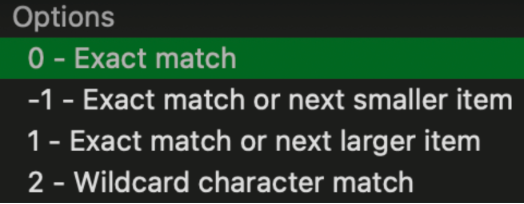
Example
=XLOOKUP(F16,$E$10:$E$12,$F$10:$F$12,,-1)
Reason #2: Stable cell reference changes
If you’ve worked with the VLOOKUP for a while, you know that the most annoying thing that happens is when you add or remove a column, the cell reference changes or errors out. To solve for this, the INDEX MATCH was introduced. While the INDEX MATCH is a good solution, it can be confusing for beginners and too long to type out for power users.
The XLOOKUP has the cell reference safety of the INDEX MATCH and the simplicity of the VLOOKUP.
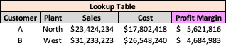
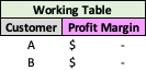
VLOOKUP / XLOOKUP Before Adding a Column

VLOOKUP After Adding a Column
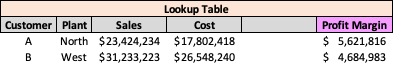
XLOOKUP After Adding a Column
Reason #3: Logical argument flow
With the VLOOKUP and INDEX MATCH options below, there wasn’t a logical argument flow.
For example, the VLOOKUP asked for the table array which had to include the lookup value always in the starting position (1) of the table array. The formula then had you give the column index number, which, as we saw in the previous reason, could easily be moved, causing an error. The VLOOKUP had so much room for misinterpretation, cell reference, and fat finger errors.
The INDEX MATCH, on the other hand, worked great, but trying to explain this concept to a beginner was tough “Yeah, you start with one formula that asks for an array and then you put in another formula as the array…”.
The XLOOKUP’s syntax and argument flow simply makes sense — what is your lookup value, what is the lookup array that contains your lookup value, what is the return array that has your desired value, do you want to build in an IFERROR value, and would you like matching and searching options.
Syntax Comparison


The XLOOKUP is the undeniable queen/king of the lookup!